Importance Sampling: Why Where You Sample Matters More Than How Much
Why is it important to know?
When you can’t solve something exactly—or it would take forever—sometimes the smart move is to ask the right questions randomly and see what answers you get. This is the essence of Monte Carlo methods: using randomness to approximate what’s too expensive or difficult to evaluate exactly. These principles are everywhere from financial modeling and machine learning to physics simulations and, yes, computer graphics.
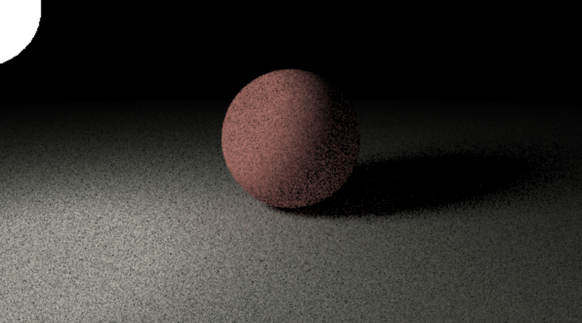
In graphics specifically, whether you’re building a game engine, a renderer, or even just tweaking shaders, you’ve probably run into the problem of noisy renders. You know, those grainy, speckled images that look like someone sprinkled digital sand all over your beautiful scene. Noise isn’t just an aesthetic problem—it’s a computational one.
The techniques we’ll talk about here, particularly importance sampling, are the difference between a render taking hours to look decent and one that looks pretty good in minutes.
For tech artists, understanding these concepts means you can make smarter choices about where to spend your computational budget. For engineers, it’s the foundation of building efficient rendering pipelines which don’t make your GPU cry. Plus, there’s something deeply satisfying about understanding why your renders look the way they do.
What is Monte Carlo Sampling?
We can think of Monte Carlo Sampling as a way to figure out the shape of really complicated integrals. It can be used to solve many kinds of integrals—even simple ones—but for our purposes, Monte Carlo shines when figuring out the value under the curve of a function that would be difficult to solve by hand. Like the rendering equation:
\[L_o(\mathbf{x}, \omega_o) = L_e(\mathbf{x}, \omega_o) + \int_{\Omega} f_r(\mathbf{x}, \omega_i, \omega_o) L_i(\mathbf{x}, \omega_i) (\mathbf{n} \cdot \omega_i) \, d\omega_i\]Don’t worry if this looks intimidating—we’ll break it down later. For now, just know the function describes how light bounces around a scene, and the integral over all possible light directions is exactly the kind of problem Monte Carlo is perfect for solving.
Here’s an example: Imagine the route you take to work or school or your favorite coffee shop each day. You might already be thinking of the amount of time the route usually takes you. Of course, this can change from a number of variables like the time of day, weather, or the timing of traffic lights.
Say we wanted to find the true average amount of time the route takes you. You’ve probably guessed that we can solve this problem using Monte Carlo. We can measure the time it takes us every day over the next month. Then, we can add up all those times and divide by the total amount of days we measured for. At the end, we’ll get an average time for this route. Note that it might not be the true average. But, rest assured that the more samples we take, the closer we will converge.
At its core, Monte Carlo integration is beautifully simple. Say we want to find the integral of some function $f(x)$ over a domain. Instead of solving it analytically (which might be impossible or really hard), we can estimate it by taking random samples. The basic Monte Carlo estimator looks like this:
\[I \approx \frac{1}{N} \sum_{i=1}^{N} \frac{f(x_i)}{p(x_i)}\]Here, $N$ is the number of samples we’re taking, $x_i$ are our randomly chosen sample points, $f(x_i)$ is the value of our function at those points, and $p(x_i)$ is the probability density function (PDF)—this tells us how likely we are to sample each point. The PDF is crucial—it’s how we account for sampling some regions more than others.
If we’re sampling uniformly (every point has an equal chance), then $p(x_i)$ is just a constant, and the equation simplifies. But as we’ll see, uniform sampling isn’t always the best strategy. The cool thing is, as $N$ gets larger, this estimate converges to the true value of the integral. Like the route time example—the more days you measure, the closer you get to the real average.
Randomness and Lighting
Now that we understand the basics of Monte Carlo, let’s see how it applies to rendering. We can take this approach a step further when simulating an environment with lighting.
Imagine a room with a ball inside. Depending on the position of the ball, we get shadows as well as brighter areas in the environment. What’s happening at the physical level? In essence, the room is flooded with light bouncing in all different directions and eventually reaches your eyes. This is literally how we see at all (remember this for later).
Decades ago, computer scientists asked the question of how they could simulate the way light bounces around an environment using the power of a computer. Let’s put ourselves in their shoes and think through how we might solve this problem. Here are some questions we might start with: Why are some areas brighter and why are some darker? How would things look if the ball was made of rubber or metal? How do we even define what light is?
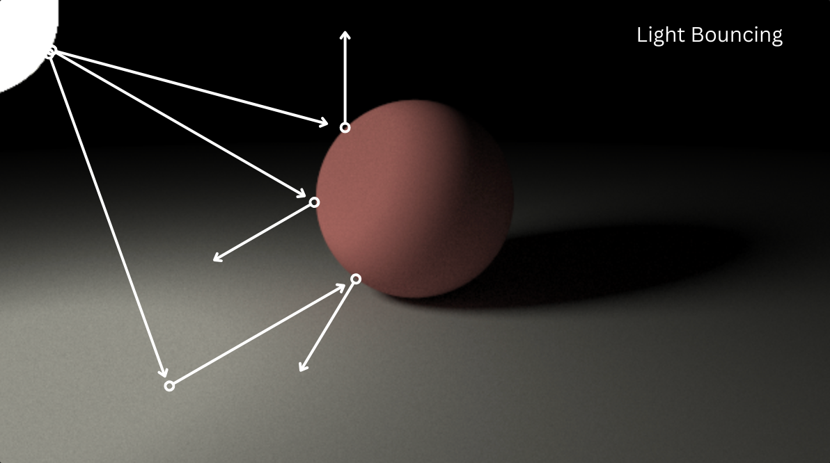
Let’s put the last question to the side for a second. Say we already have a way to define what a light is (like perhaps a ray). If everything we see is defined by the light entering into the environment, bouncing around, then reaching our eyes, why don’t we just account for all of those light rays and all the different angles they can bounce in, then put that all together?
This would, theoretically, be the exact way to simulate our scene. However, remember we are using a computer. Accounting for the amount of light rays bouncing around, the number of bounces they might do, and the different directions they might go in would be extraordinarily expensive. We may need something like a beta version of Laplace’s demon to render this scene in a timely manner.
So, okay. Say we want to render this within our lifetimes. We have to look at another method (you guessed it). This is the cool thing about Monte Carlo. Remember in the average route time example? You didn’t have to measure all the times you’ve taken that route. Just some amount to be representative enough to get a good idea of the average time. The cool thing is that the more simulations you run with Monte Carlo, the closer you’ll get to the true average.
Remember the rendering equation from earlier? That’s essentially the equation that accounts for all the ways that light and materials interact in an environment. It looks super daunting. But, it can be broken up into 3 simple components:
- The amount of light coming in
- How much light is absorbed/reflected
- The angle of the incoming light
The integral is a representation of the fact that we are summing up the product of each of these components for every ray of light that’s hitting the sphere from all possible angles. Now, if we could evaluate this equation for all points on the sphere and all angles the lights could go, then we could just use that to simulate the light in our environment.
The thing is, we don’t and we can’t because we’d have to know it for an infinite amount of directions that light would be coming from for just a single point. Luckily, we don’t have to know all this. We can just randomly sample different directions that the light can go in using Monte Carlo simulations. The average of these simulations will approximate the rendering equations more and more closely as we take more and more samples.
However, this process is also flawed. If we sample randomly, we’ll sample a lot of directions that just don’t matter, which means that we waste precious compute.
Variance in Ray Sampling
This inefficiency shows up in our renders as variance. Variance is Monte Carlo’s way of telling you how uncertain—and therefore how noisy—your estimate is.
Think of it like this: if you’re trying to figure out the average height of people in a city, and you sample ten people who all happen to be professional basketball players, your estimate is going to be way off. That’s high variance—your samples aren’t representative of the whole population.
In rendering, variance shows up as noise. When you randomly sample light directions, some of those samples might hit bright light sources (contributing a lot to the final color) while others hit dark corners (contributing almost nothing). The more this variation between samples, the more variance you have, and the noisier your image looks.
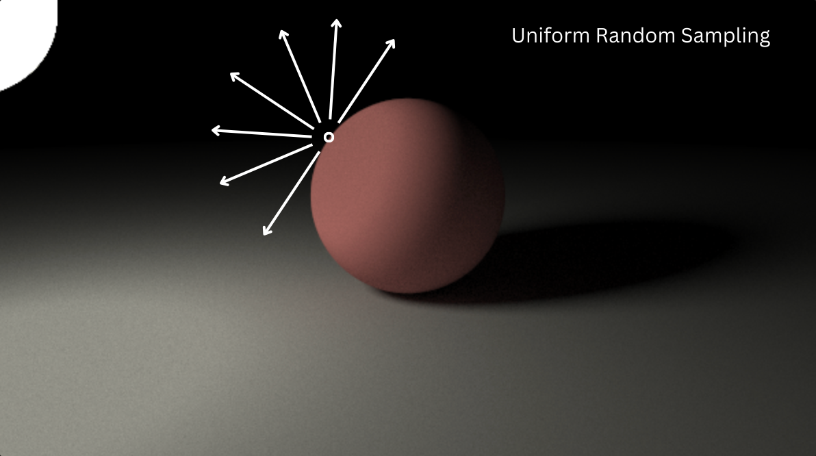
Here’s the thing about light though: it’s not uniform. As I said before, some directions matter way more than others. Light coming directly from a bright lamp matters a lot more than light coming from a dark corner of the room. When we sample randomly, we’re treating all directions as equally important, which means we’re wasting samples on directions that barely contribute to the final image.
This is where variance becomes our teacher—it’s telling us that we’re asking the wrong questions. Instead of “what if we sample this random direction?” we should be asking “which directions actually matter for this pixel?” Variance is essentially the universe’s way of pointing out that we’re being inefficient. The lower the variance, the fewer samples we need to get a clean image, and the faster our renders complete.
How do we know which directions to sample?
This is where importance sampling comes in. The key insight is that we should spend more of our computational budget on directions that actually contribute to the final image. But, how do we know which directions are important?
The answer lies in understanding what makes a direction “important” in the first place. For lighting, a direction is important if it contributes significantly to the final color of a pixel. This could be because there’s a bright light source in that direction, or because the material at that point reflects light strongly in that direction, or both. The rendering equation mentioned earlier actually tells us this—it’s the product of the incoming light, the material properties, and the geometry.
So instead of sampling uniformly across all possible directions, we can sample according to a probability distribution that matches (or at least approximates) where the light is actually coming from. If we know there’s a bright light source in a particular direction, we can create a sampling distribution that’s more likely to sample in that direction. This is like the difference between randomly guessing where your keys are versus having a general idea of where you usually leave them. You’re still not guaranteed to find them immediately, but you’re much more likely to find them faster.

The tricky part is that we need to account for this non-uniform sampling in our Monte Carlo estimator. Remember that PDF term $p(x_i)$ from earlier? When we sample more in certain directions, we need to divide by the probability of sampling those directions to keep our estimate unbiased. It’s like if you’re more likely to sample certain areas, you need to weight those samples down accordingly, otherwise you’d be overcounting them.
But wait—what happens if we get this wrong? This brings us to another important concept: bias.
How do we account for bias?
Bias is Monte Carlo’s sneaky cousin. While variance tells us about the uncertainty in our estimate, bias tells us if our estimate is systematically wrong. An unbiased estimator will, on average, give you the correct answer. A biased estimator will consistently give you an answer that’s off in one direction—always too high or always too low.
When we do importance sampling correctly, we maintain an unbiased estimate. That’s why we divide by the PDF term; it keeps us honest. By dividing by the probability of sampling each direction, we’re essentially saying “we sampled this direction more often, so we’ll weigh it less to compensate.” This ensures that even though we’re sampling non-uniformly, our final estimate still converges to the true value.
Bias can still creep in if we’re not careful, though. If our sampling distribution doesn’t match the actual distribution of light in the scene, or if we make mistakes in how we calculate the PDF, we can introduce bias. For example, if we sample toward a bright light source but forget to properly account for the probability of sampling in that direction, we might overestimate the brightness.
With proper importance sampling, we can reduce variance (less noise) without introducing bias (still getting the right answer on average). It’s the best of both worlds: faster convergence to the correct result. The trade-off is that importance sampling can be more complex to implement—you need to figure out good sampling distributions and calculate PDFs correctly. But the performance gains are usually worth it.
In practice, most modern renderers use a combination of techniques: they might importance sample based on the material’s BRDF (Bidirectional Reflectance Distribution Function—essentially how the material reflects light), or based on the light sources in the scene, or both. The goal is always the same: sample more where it matters, account for it properly, and get cleaner images faster.
Approximating the Rendering Equation with Monte Carlo
As we went over before, the rendering equation describes how light interacts with surfaces in a scene.
\[L_o(\mathbf{x}, \omega_o) = L_e(\mathbf{x}, \omega_o) + \int_{\Omega} f_r(\mathbf{x}, \omega_i, \omega_o) L_i(\mathbf{x}, \omega_i) (\mathbf{n} \cdot \omega_i) \, d\omega_i\]Where $L_o$ is the outgoing radiance (the light leaving a point in a direction), $L_e$ is the emitted light (if the surface itself is a light source), $f_r$ is the BRDF (Bidirectional Reflectance Distribution Function—how the material reflects light), $L_i$ is the incoming light, and $(\mathbf{n} \cdot \omega_i)$ is the cosine term that accounts for the angle between the surface normal and the incoming light direction. The integral is over the hemisphere $\Omega$ of all possible incoming directions $\omega_i$.
Now, here’s where Monte Carlo comes in. We can’t solve this integral analytically because it’s too expensive, so we estimate it by sampling. The Monte Carlo estimator for the rendering equation becomes:
\[L_o(\mathbf{x}, \omega_o) \approx L_e(\mathbf{x}, \omega_o) + \frac{1}{N} \sum_{i=1}^{N} \frac{f_r(\mathbf{x}, \omega_i, \omega_o) L_i(\mathbf{x}, \omega_i) (\mathbf{n} \cdot \omega_i)}{p(\omega_i)}\]This is saying: for each sample direction $\omega_i$ we randomly choose (according to our sampling distribution $p(\omega_i)$), we calculate how much light is coming from that direction, how the material reflects it, account for the angle, and then divide by the probability of sampling that direction. We do this $N$ times and average the results. As $N$ increases, this estimate gets closer and closer to the true value of the integral.
The beauty of this formulation is that it works regardless of how we choose our sampling distribution $p(\omega_i)$. If we sample uniformly, $p(\omega_i)$ is constant. If we do importance sampling, $p(\omega_i)$ varies, but the estimator remains unbiased as long as we divide by the PDF correctly. This is the mathematical foundation that makes importance sampling possible—we can be smart about where we sample, as long as we’re honest about how we’re sampling.
Putting It All Together
So what have we learned? Monte Carlo sampling gives us a way to approximate complex integrals—like the rendering equation—by taking random samples. But not all samples are created equal. Some directions contribute more to the final image than others, and randomly sampling everything equally leads to noisy, inefficient renders.
Importance sampling solves this by concentrating our computational budget on directions that actually matter. We sample more where light is bright or where materials reflect strongly, and we account for this non-uniform sampling by dividing by the PDF to keep our estimates unbiased. The result? Cleaner images in less time.
The key insight is that variance isn’t just noise—it’s feedback. It tells us we’re asking the wrong questions. Instead of “what if we sample this random direction?” we should be asking “which directions actually matter?” When we listen to that feedback and sample accordingly, we get the best of both worlds: reduced variance (less noise) without introducing bias (still getting the right answer).
Whether you’re optimizing a renderer, tweaking shaders, or just curious about how modern graphics work, understanding importance sampling gives you the tools to make smarter choices about where to spend your computational budget. And that’s the importance of asking the right questions.