Rendering a Simple Iridescent Material

A Simple Iridescence Algorithm

There are many examples of iridescent materials in the real world. Bubbles, oil in water, bismuth. What gives them their colorful complexion? It turns out the physical phenomena at play is pretty complicated (For those who want to do a deep dive). For the sake of simplicity, what we see is a mixture of different color frequencies, where that mixture changes depending on the angle we are viewing the object from. Thankfully, there are simpler methods to approximate this behavior. I’m gonna go over the one I’m using in my Ray Tracer here.

The Method

It helps to think about what considerations we need to make. In our model for simulating the effect of iridescence, we have to consider the angle we are viewing the object from, the different color frequencies, and how they “mix” based on that angle. As far as angle is concerned, we focus on two components: the direction we are viewing the object from, and the normal at the point on the surface being viewed. We then compare the angle between these two, in order to get an idea of what the reflected color should be.

To do this comparison, we turn to linear algebra. Let’s create two rays from the surface of our material: $\mathbf{V}$ for the direction from a point on the object toward the viewer, and $\mathbf{N}$ for the normal at that point. Assuming both are normalized, we can get the cosine of the angle between them using the dot product.

\[\cos(\theta) = \mathbf{V} \cdot \mathbf{N}\]

Next, we want a way to map this angle to an output in the form of color. Lets first start with our different color frequencies. Let $\mathbf{F}_r$, $\mathbf{F}_g$, and $\mathbf{F}_b$ be the frequencies for the Red, Green, and Blue color channels, respectively. I’ll refer to them collectively as RGB waves. The color changing effect we see when moving an iridescent object around occurs as a consequence of changing our viewing angle. At each viewing angle, we get a different mix of RGB waves producing a different overall color.

The reason we get a different mix comes down to wave interference. Red light has the longest wavelength, green has a medium wavelength, and blue has the shortest wavelength. When light reflects off the surface at different viewing angles, the path length differences cause the RGB waves to shift out of phase with each other. Sometimes these waves constructively interfere (amplifying each other), and sometimes they destructively interfere (canceling each other out). This phase-dependent interference is what creates the shifting color gradient we see as we move an iridescent object around.

Figure 1

For example, note the different viewing angles in Figure 1. At each viewing angle $\theta$, the path length that light travels changes, which shifts where we sample each RGB wave in its cycle. This means that at viewing angle $\theta_1$, we might sample all RGB waves at points where their peaks align (constructive interference), creating a bright red-green-blue mix. At a different viewing angle $\theta_2$, the phase relationships change: now $\mathbf{F}_g$ and $\mathbf{F}_b$ might be out of phase (destructive interference), dampening their contribution, while $\mathbf{F}_r$ could be at its peak, making red more prominent. This phase-dependent sampling is what creates the smooth color gradient as we change our viewing angle.

Mapping Angle to Phase

Now, to map the viewing angle to the cosine phase value, we need a way to introduce the gradient as the angle of view grazes the object more and more. Think about a bubble. When looking straight at it, we can see one or two colors in the middle. But, off to the side (as the viewing and normal separate) we start to see the color gradient as the different colors squish closer together.

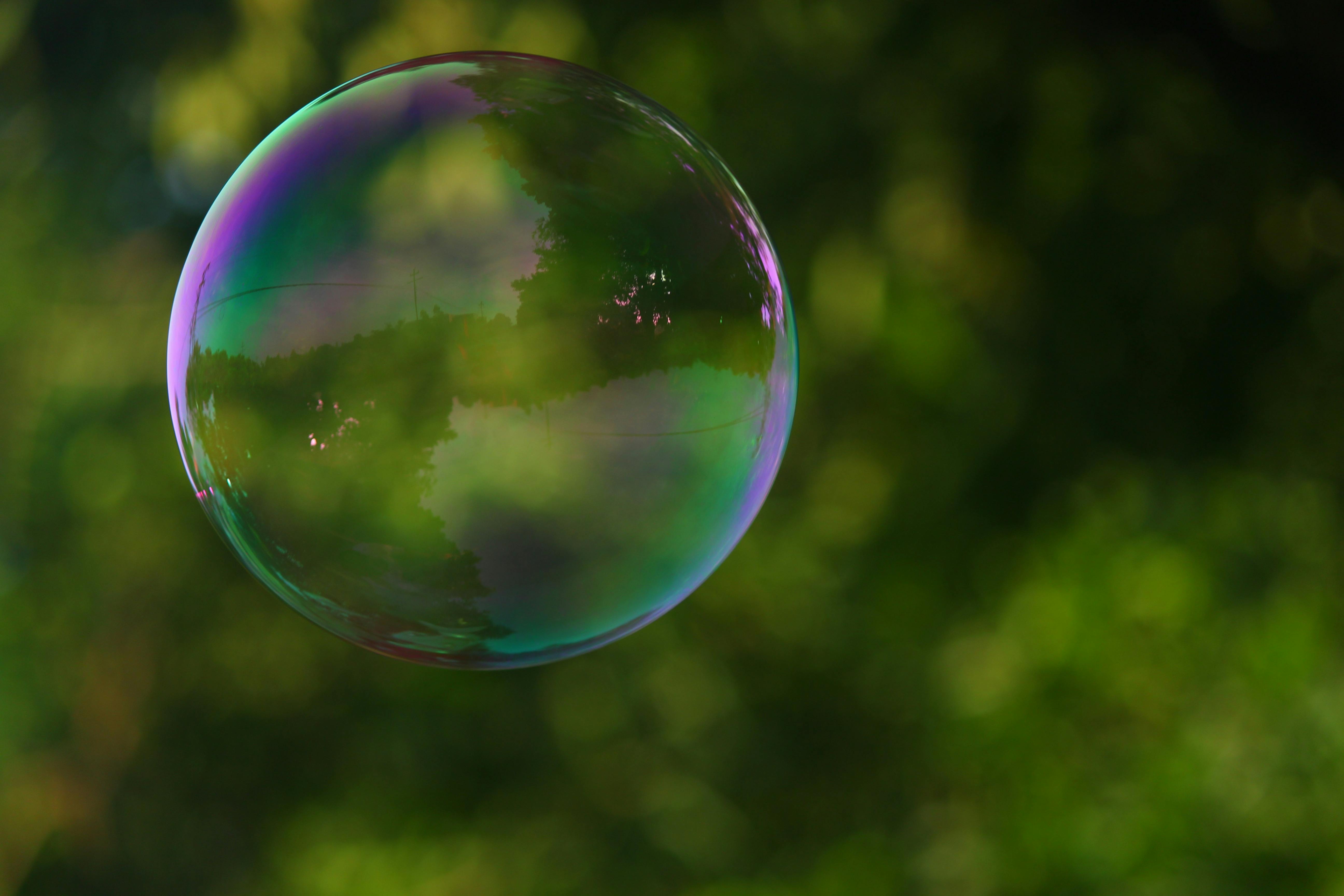
Figure 2

We start by mapping $\cos(\theta)$ to a value that increases as we move away from the normal. Since $\cos(\theta)$ ranges from 1 (looking straight at the surface) to -1 (grazing angle), we can transform it:

\[x = 1 - \cos(\theta)\]

This gives us a value that ranges from 0 (normal viewing) to 2 (grazing angle). We then multiply this by a constant $k$ to control how many color bands we see:

\[\text{phase} = k \cdot x\]

The parameter $k$ determines the number of color cycles we’ll see as we rotate the object. A larger $k$ means more bands and more rapid color changes. In practice, values around 6.0 work well for most materials.

Modeling Wave Interference with Cosine

Now that we have a phase value, we need to model how the RGB waves interfere with each other at different phases. This is where the cosine function becomes our tool of choice.

Recall that cosine functions naturally model wave behavior. When two waves are in phase, their values add constructively. When they’re out of phase, they cancel each other out. By using cosine functions with different frequencies for each color channel, we can simulate how red, green, and blue waves shift in and out of phase as the viewing angle changes.

We define frequency multipliers for each color channel:

• $f_r = 1.0$ (red)
• $f_g = 1.3$ (green)
• $f_b = 1.7$ (blue)

These values are chosen to create distinct phase relationships between the channels. Notice that green and blue have higher frequencies than red, which means they’ll cycle through their interference patterns more rapidly as the phase changes. This creates the characteristic color-shifting effect where different colors become prominent at different viewing angles.

The Color Calculation

For each color channel, we calculate its intensity using a cosine function:

\[R = 0.5 \cdot (1.0 + \cos(f_r \cdot \text{phase}))\] \[G = 0.5 \cdot (1.0 + \cos(f_g \cdot \text{phase}))\] \[B = 0.5 \cdot (1.0 + \cos(f_b \cdot \text{phase}))\]

The formula $0.5 \cdot (1.0 + \cos(…))$ normalizes the cosine output (which ranges from -1 to 1) to a value between 0 and 1, suitable for color channels. When $\cos(f \cdot \text{phase}) = 1$, the channel is at maximum intensity. When $\cos(f \cdot \text{phase}) = -1$, the channel is at minimum intensity.

Because each channel uses a different frequency multiplier, they’ll peak and trough at different phase values. This means at any given viewing angle, one color might be bright while another is dim, creating the iridescent color gradient we’re after.

Blending with Base Material

In practice, iridescent materials often have a base color or material underneath. For example, a soap bubble has a transparent base, while an iridescent paint might have an underlying color. We can blend the iridescent effect with a base material using a strength parameter:

\[\text{final color} = (1 - \text{strength}) \cdot \text{base color} + \text{strength} \cdot \text{iridescent color}\]

When $\text{strength} = 0$, we get only the base material. When $\text{strength} = 1$, we get only the iridescent effect. Values in between create a subtle blend, which is often more realistic for many materials.

The Algorithm

Putting it all together, here’s the complete algorithm for computing an iridescent color:

function iridescent_color(view_direction, surface_normal, base_color, strength, k, fr, fg, fb):
    // Step 1: Calculate viewing angle
    cos_theta = dot(view_direction, surface_normal)
    
    // Step 2: Map angle to phase
    x = 1.0 - cos_theta
    phase = k * x
    
    // Step 3: Calculate RGB intensities using cosine interference
    R = 0.5 * (1.0 + cos(fr * phase))
    G = 0.5 * (1.0 + cos(fg * phase))
    B = 0.5 * (1.0 + cos(fb * phase))
    
    iridescent_color = (R, G, B)
    
    // Step 4: Blend with base material
    final_color = (1.0 - strength) * base_color + strength * iridescent_color
    
    return final_color

Parameters:

• k = 6.0: Controls number of color bands
• fr = 1.0, fg = 1.3, fb = 1.7: Frequency multipliers for RGB channels
• strength: Blend factor between base material and iridescent effect (0.0 to 1.0)

This algorithm captures the essence of iridescence: the angle-dependent phase relationships between different color frequencies, modeled through simple cosine functions. The result is a smooth, realistic color gradient that shifts as you move around the object, just like real iridescent materials.

Result

Implementing this into my ray tracer, I get the following:

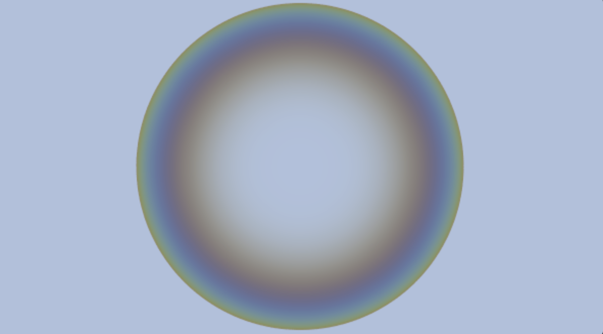
Figure 3

Not bad. Hope you learned something!